1. Introduction

The goal of the project is to implement an image classification system. The main task is to train image classifiers on the Training set, and do the testing on the Testing set. A dataset is provided, which contains 5 classes ("bedroom", "industrial", "kitchen", "living room", "store").

2. Resources

In this project, we have implemented a image classification based on the skeleton code provided. The system is programmed in MATLAB. Some third-party libraries were also used to promote the performance. Download links of the code and other libraries are listed here

1) Project Code (alternative download:dropbox)

2) VL_Feat (Feature Extraction Library)

3) LibSVM (High Performance SVM Implementation)

4) LibLinear (Large Scale Linear SVM)

5) Sparse Coding(OMP Sparse Projection, SPAM)

6) LLC coding (local constraint linear coding)

3. System Framework

The system consists of three parts: 1) Feature Extraction Module; 2)Image Representation Module; 3)Classifier Module. Based on these modules, we implemented a complete pipeline from input image to classification result, and can evaluate the performance of our algorithm by the classification accuracy.

3.1 Feature Extraction

We have tried a few image features, including dense sift, surf, and gist. The best feature selection we found is the dense sift with gist. To our understanding, the gist feature reveal the local detail of the image, while the gist feature gives an holistic decription of the image. The dense sift feature is extracted using VL_Feat library. In the extraction process, we set the spacing of the dense grid to 6 pixels, and the sampling window is set to 16*16 pixels.

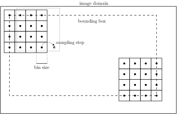
Figure 1 Dense Grid to Extract DSIFT

The gist feature is a well-developed feature used in scene recognition. It uses Gabor filter to extract a holistic description of a lot properties of the image. These properties are highly related to the underlying scene where the image was taken. It will help determine what type of object the image is showing. However, the images we used in the experiment are only grayscale images, which will constraint the performance of the gist feature. But gist feature actual improves our recognition performance.

3.2 Image Representation

3.2.1 Feature Coding

After feature extraction, we get the raw form of feature descriptors. These descriptors cannot be directly used in recognition. We do a coding processing on the descriptors to get the final image representation for recognition. Here we also tried a few methods. We set the codebook length to 1500 and tried these coding method: 1)nearest neighbor and k-NN 2)LLC (local linear constraint coding) 3)sparse coding. These method has variant performance on the dataset. The best performance is achieved with LLC.

In the experiment, the coding is committed on dense sift features. In the training process, we extract a dataset of about 350 thousands descriptor vectors. Then we try to learn a codebook of 1500 vectors from the dataset. The learning here we used is kmeans for NN and LLC, and sparse dictionary learning for sparse coding (using SPAM software).

a) Nearest neighbor method

In the nearest neighbor method, to code a feature vector, we find its 1 or k nearest neighbors in the codebook. Then we use the Gaussian kernel similarity metrics to represent this vector by codebook.

b) LLC

The local linear constraint coding is a fast coding method. Using the kmeans result for the code book, we achieved a good recognition performance. We have modified the original code to adapt to our usage.

c) Sparse Coding

Sparse coding method is a novel concept raised in recent years. It aims to represent an input with sparse composition of a codebook set.

3.2.2 From code vector to representation

After we code the descriptor vectors, we still have a lot of code vector, we still have a lot of vectors with one image. Commonly, we can make a histogram by sum up vectors of one image. However, a direct histogram loses spatial information of these descriptors, which may be very important for recognition. To preserve spatial relations of the code vectors, we introduced the spatial pyramid matching techniques. Pooling is also used, which is like the way biological visual system does.

Spatial pyramid match aims to preserve the spatial relationship between local descriptors. The basic idea is to divide the image into a few rectangle blocks and do the histogram in the block. In layer of the pyramid, the image is equally divided into blocks. Each block has a histogram of codes. Thus the image is represented by a vector, where is the length of the codebook. The emphasize the importance of the spatial position, histogram of each layer is assigned with a weight , where L is the number of layers.

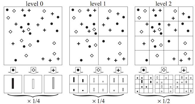
Figure 2 Spatial Pyramid of 3 Layers

Pooling is a concept comes from biology neuroscience. Instead of histograming, pooling method apply a function on each element of all code vectors in the dataset, which lead to a value assigned to the corresponding element in the representation vector. Experiments shows that pooling can improve the result of LLC and sparse coding.

3.3 Classfiers

The image representation we obtained need to be fed to a set of classifiers to determine their classes. In this project, I used the LibLinear library, a SVM library used for large-scale data. This library is very suitable for our mission, which needs a fast classifiers to handle the long feature vector given by spatial pyramid technique. Our problem can be formulated as a multi-class classification problem. We choose the one-vs-all strategy to train the SVM. This means we train n SVMs, each labels the sample inside one class as +1 and other samples as -1, in total we have n classes. In classification, the test sample will be fed to n classifiers, the highest score given by classifier i means the sample belongs to class i.

4. Experiments

4.1 Results

We do experiments on the data given. The training set has 5 classes, each has 60 images. The testing set has 5 corresponding classes, each has 40 images. To test the performance of our algorithm, we train our codebook and classifiers on the training set. Then we permute the testing set to a set of 200 images, their class label are saved in the ground truth file. Then we calculate the recognition accuracy on the testing set. The experiment results are shown below. Note the spatial pyramid is set to 3 layers, and the pooling is max-pooling.

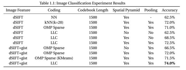
Figure 3 Image Classification Result. Here LLC use 20 nearest neighbors.

We can see that the best performance is obtained using dSIFT with gist features, LLC coding and a 1500 entries codebook. The best recognition accuracy was 74%.

4.2 Discussion

We have discussed in previous section that dSIFT adding gist can give us a local and global representation of the image scene. We It is not so trivial that LLC, sparse coding, and kNN are on par with each other in performance. One possibility is that the codebook of 1500 words may have mostly covered the image visual sementics.

One interesting fact is that when we use the KMeans codebook to do the sparse coding experiment, performance only slightly decreased. We suggest that the sparse coding result is not so dependent on the codebook learning method. But it is more related to the sparse model. When we use the Homotopy solver to do the sparse coding, we achieved a result that is even lower than our baseline, the nearest neighbor hard coding.

Another important fact is that spatial pyramid matching and pooling can significantly improve the performance of both LLC and sparse coding. For LLC, the improvement of pyramid with pooling is about 10%. For sparse coding, the improvement from pyramid matching (pooling is default for sparse coding) is about 5.5%. This shows that spatial information is important for recognition.

5 Conclusion

In this project, we built up a image classification system use various features, codebooks and coders. We also test the importance of spatial pyramid matching and pooling. Finally the best recognition rate we achieved is 74%. In the implementation, the feature extraction, sparse coding and classifiers are from 3-rd party libraries, other part of the system are all implemented by myself based on the structure of given skeleton code.

Reference

[1] R.-E. Fan, K.-W. Chang, C.-J. Hsieh, X.-R. Wang, and C.-J. Lin. LIBLINEAR: A Library for Large Linear Classification, Journal of Machine Learning Research 9(2008), 1871-1874.

[2] Andrea Vedaldi and Brian Fulkerson. 2010. Vlfeat: an open and portable library of computer vision algorithms. In Proceedings of the international conference on Multimedia (MM '10). ACM, New York, NY, USA, 1469-1472.

[3] Lazebnik, S.; Schmid, C.; Ponce, J., "Beyond Bags of Features: Spatial Pyramid Matching for Recognizing Natural Scene Categories," Computer Vision and Pattern Recognition, 2006 IEEE Computer Society Conference on , vol.2, no., pp.2169,2178, 2006

[4] David G. Lowe, "Distinctive image features from scale-invariant keypoints," International Journal of Computer Vision, 60, 2 (2004), pp. 91-110.

[5] Oliva A, Torralba A. Modeling the shape of the scene: A holistic representation of the spatial envelope. International journal of computer vision, 2001, 42(3): 145-175.

[6] Wang J, Yang J, Yu K, et al. Locality-constrained linear coding for image classification. Computer Vision and Pattern Recognition (CVPR), 2010 IEEE Conference on. IEEE, 2010: 3360-3367.

[7] Allen Yang, Arvind Ganesh, Zihan Zhou, Shankar Sastry, and Yi Ma. Fast L1-Minimization Algorithms for Robust Face Recognition. (preprint)

[8] J. Mairal, F. Bach, J. Ponce and G. Sapiro. Online Learning for Matrix Factorization and Sparse Coding. Journal of Machine Learning Research, volume 11, pages 19-60. 2010.

Appendix A: How to setup and run the matlab package

1. Install and run

On installing, just extract the package to any place you want. To test the recognition performance, just put the test images into the “/testing” folder just as the current images does, every class has its pictures in the subfolder of the class id (0,1,2…). Then run the matlab script “image_classification_system.m” you will see the result when script runs to an end. Note that the order of test image will be uniform random permuted.

2. Program setup

The package contains a standard configuration file “config.ini”. The content of the file and the setting we used to achieve the best performance is listed below:

If the image numbers every class in testing set is changed, please set the parameter “nImgPerClass_testing” to the actual number you are using. This package also contain pretrained codebooks using kmeans and sparse dictionary learning. If you want to train your own codebook, please change the value of “trainBook” to ‘true’.